Abstract

Fantasy Football is the most popular fantasy sport in the United States with estimates of 33 million participants every year.  In addition to league fees that are paid to internet providers, many leagues have their own pool of money with the winner taking the lion’s share.  The Fantasy Sports Trade Association (FSTA) estimated in 2013 that $1.18 billion changes hands within leagues every year (Green, 2014).  In addition to the financial stakes is personal pride; no one wants to lose. 

In order to gain an edge on their fellow fantasy league managers, team managers can turn to many web sites for guidance.  A simple search on bing.com returns 63,000 results for the term “Fantasy Football 2014 Rankings.”  There is no shortage of sites offering advice on how to draft, who to draft, and when to draft.  At the core of this process is estimating how much a given player will score in each game and over the course of a season.

This paper discusses techniques for using Vectorial ARMA models to improve the predictions of quarterback fantasy statistics.

 

 

Introduction

Fantasy football began in 1962 when Wilfred Winkenbach with some colleagues developed a system and rules that led to the formation of modern fantasy football (Hunt, 2014).  The growth of the game was slow due to the manual nature of entering and keeping track of scores.  The growth of fantasy football took off in the late 1990’s when the popularity of the internet and the automation of administrative duties made it possible for millions of fans to just choose their teams without having the administrative burden.  Today, 33 million people play every year. 

In fantasy football regular people get to pretend to be team owners.  They choose their players and assemble a team of stars.  A group of friends can form a league and compete against each other.  Typically they pay a website an annual fee to host the league and draft process and compete against each other in a round-robin format for the first 12 or 13 weeks of the season.  At the end of the 12 weeks, the top four teams go into the playoffs.  The best teams compete against each other in multi-week rounds, and in the 16^th week, the league champion is crowned.  There are 17 weeks in the NFL season, but most leagues stop after 16 because many stars do not play the 17^th week if their teams have already secured a spot in the real playoffs. 

Fantasy teams score points by accumulating various statistics from the real-life performances of players on the field.  Each team usually includes a quarterback, three wide receivers, two running backs, a tight end, a kicker, and a defense (an entire team is chosen).  An entire team is made up of 16 different players, and the manager selects which players will “play” each week.  If the active players score certain statistics, their managers are rewarded with points.  The team with the most points wins the matchup and each manager accumulates a win-loss record, which makes him/her eligible for the playoffs and a portion of the league payout. 

The team manager chooses the players on their team through a draft process.  The two common draft procedures are the snake draft and the auction draft.  In the snake draft, the managers take turns making picks.  Prior to the draft an order is set.  To make the draft process fair, the manager that picked first in the first round, picks last in the second round, and then picks first again in the third round, etc.  The image below shows a typical snake draft.

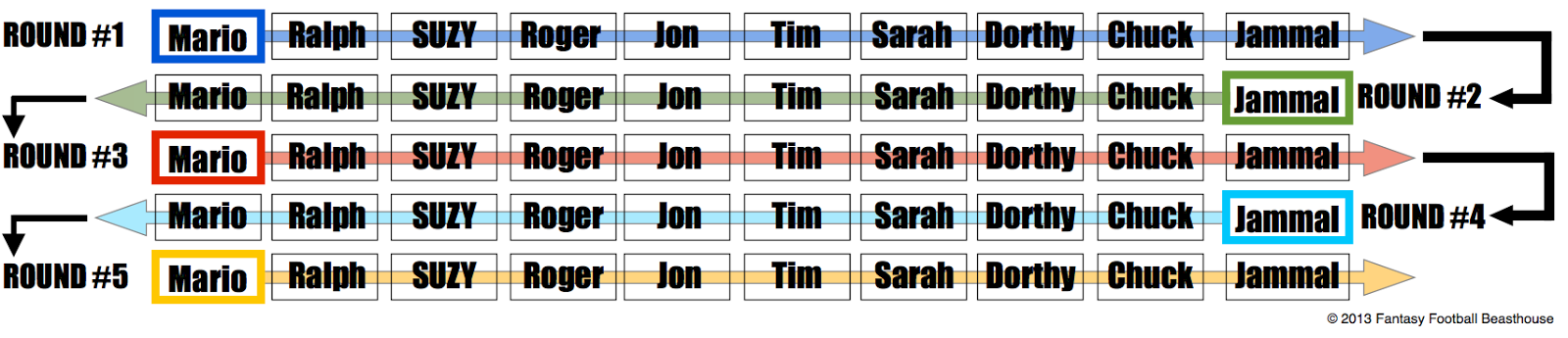
In a snake draft it is important to choose the player that will improve the team’s performance the most that is not likely to be available the next time the team manager is able to draft.  Determining which players will not be available gets more difficult in later rounds, but it does not matter as much either.  The marquee players always go in the first two or three rounds.  Even if an estimate of a player’s worth is off a few positions the player is still not likely to be available the next time the manager drafts.  In many leagues, certain positions will not be taken before certain rounds.  So even if a player is more valuable, it helps to know that he may be available the next round, and can be safely undrafted until the next opportunity arises.

The alternative type of draft is the auction draft.  In an auction draft, each player receives a budget, similar to the NFL’s salary cap.  The manager’s take turns choosing a player and the managers bid on the player.  The highest bid for a player wins.  There is a strategy involved in this method as well.  It may be that one manager wants to force another manger to overbid on a certain player.  This will consume more of the opposing manager’s budget and lower the price for following players.

Fantasy football, like other fantasy sports, allows the fans to more actively participate in the sport.  Whereas in the days before fantasy football most fans knew about their own team, and could name a few stars from the rest of the National Football League (NFL), fantasy football requires a deeper knowledge of the players in the league.  In a league with 12 teams and 16 players per team, team managers need to know at least 192 of the players in the league.  It also means that on any given night, a team manager will have a rooting interest in several other games.  This is good business for the NFL.

For the team managers, being good at fantasy football means the owner knows more about football than the other owners in the league.  Part of each year’s draft preparation is to determine which players are likely to score the most fantasy points.  Most fantasy football web sites provide their own predictions for each player.  The methodology behind these projections is opaque.  The objective in this paper is to apply time series analysis to football statistics in order to come up with better predictions and a better overall team. 

Method

The first part of this analysis was to get the data to use within MATLAB.  For this, I went to a web site called FFToday.com.  They have weekly statistics and fantasy scoring for every player at every position going back to the year 2,000.  The data is in table format.  This can be copied and pasted into Microsoft Excel, but requires manipulation within Excel in order make it ready to store in a database.  Additionally, copying and pasting the results for 14 seasons for 6 different positions would take several days and is subject to manual error.  Instead, I created a Python model that uses the built-in urllib to “screen scrape” the data and load it into a sqlite database.  This procedure could load the 14 seasons into the database in about 30 minutes.  In all, over 100,000 rows of data were downloaded. 

Given the complexity of analyzing the factors contributing to the scoring of every position, I changed the focus to just quarterbacks.  For the quarterbacks, I had 16,123 rows of data compiled by 247 different quarterbacks.  This is an average of only 65 games per player.  This is not enough data to complete a time series analysis.  Additionally, many of those players only played a few games in a season and mostly scored 0 points each game.    Only four quarterbacks had close to 200 games of history, these were Peyton Manning (195), Matt Hasselbeck (210), Tom Brady (210), and Drew Brees (195).  Given the need for close to 200 samples, and an average career that is only 1/3 of that, I searched for another method.

Rather than model each quarterback, I flipped the problem on its side.  Instead of modeling what a quarterback scored over time, I modeled what quarterbacks scored over time against a specific team.

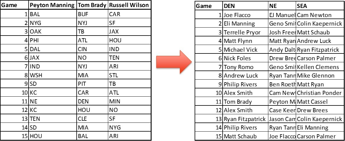
To account for the differences in the quarterbacks playing against each team, the quarterback’s average from the prior season was subtracted from the score.  I subtracted the average of the residuals to get a time series for each team with a mean of 0. 

The residuals all appear to be random data, and the correlated residuals did not show any abnormal patterns.

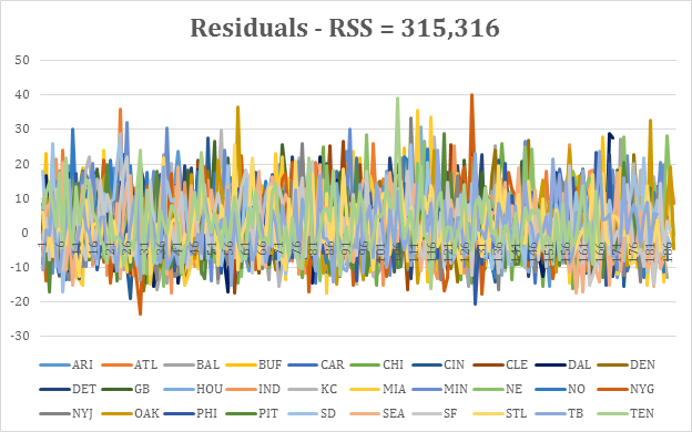
Residuals for each team

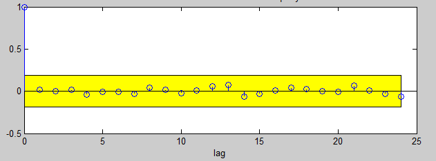
Correlated residuals for a sample team.

In order to get a base model, I ran the Postulate ARMA Matlab script.  Most models were ARMA (1,1) and typically looked like white noise.  There were some exceptions, such as Detroit, Denver, and Cleveland, which had higher order models.  The results are in Appendix B.  Given the normalizing process worked so well, so that most of the data could be seen as white noise, I modified the Postulate script to try and see if a higher MA order was possible.  After the AR order is determined, Postulate checks to see if it can reduce the MA order further.  Instead of starting from (m,n) and working back to (m,0), I made the incumbent model (m,20) and worked backwards.  In most cases the final model was still ARMA (1, 1).  One exception is Philadelphia with ARMA (3, 10).  All other examples had MA orders lower than their AR orders. 

Once the base model was determined, I experimented with using other time series to determine improve the forecast.  The potential new time series were the following:

• Sacks:  This is when the defensive team tackles the quarterback before he can pass it.  The reasoning behind its importance is that a quarterback can get hurt, and will be more cautious or throw the ball away rather than be sacked again.
• Interceptions:  This is when the defensive team catches a pass from the quarterback.  An interception affects the quarterback’s confidence and takes the quarterback off the field so he cannot score more points.
• Fumbles Recovered:  This happens when a player drops the ball and the play has not stopped, but the defense recovers the ball.
• Rushing Attempts:  This is the number of attempts by the quarterback’s team to rush the ball.  This happens when the quarterback chooses to hand the ball off instead of throwing it.  The quarterback does not accumulate any statistics when this happens.  It is less risky, but may not yield as many gains down the field.
• Rushing Touchdowns:  This happens on a rushing play and the running back scores a touchdown.  Again, the quarterback does not gain any point on this play.

Though it is likely that all five of these time series could contribute to improving the forecast of a quarterback’s scoring, I chose to only include two of the new time series in the analysis.  These were the sacks and interceptions.  These two time series are consistent from one observation to the next because it is the same defensive team responsible for the statistics.  For this analysis I used the ARMA given by the modified postulate script and changed the order for the sacks and interceptions time series inputs.

When trying to add an order one ARV term to the model for either sacks or interceptions, the results showed no improvement in the reduction of the residual sum of squares (RSS).  When combining the two, it did show some improvement, but not enough to be statistically significant.  As a result, I experimented with ARV (2, 2) and ARV (3, 3).  Both of these yielded a few significant improvements for some teams, but most teams still worked best with just their standard ARMA models and not ARMAV.  The results of the F Tests for the ARMAV examples are in Appendix A.

Results

In 2012, with the exception of the top quarterback, the difference in the average number of fantasy points scored per game by each quarterback was less than one point per game.  The average number of points scored by the number two quarterback in 2012, Tom Brady was 25.52.  The 12^th quarterback, Russell Wilson, was 20.32.  In the NFL, the schedules adjust from year to year, so that a team that did poorly the year before will face other teams that did poorly the year before.  The upcoming schedule for a quarterback can be important.  It may only affect the points by less than a point per game, but this difference can move the quarterback up or down two to three spots.  Armed with this knowledge, a fantasy football manager can pay less or draft later if he knows a player will exceed the expectations that most others have put upon him. 

The following table includes the forecasts for the top 12 quarterbacks of 2013. 

Player	Team	Actual Average	Forecast	Actual Rank	Forecast Rank
Peyton Manning	DEN	31.18667	26.49	1	5
Drew Brees	NO	26.4	28.88	2	1
Matthew Stafford	DET	23.54667	24.67	3	8
Andy Dalton	CIN	23.13333	23.19	4	10
Cam Newton	CAR	22.5	28.09	5	2
Philip Rivers	SD	22.39333	20.21	6	12
Ben Rothlisberger	PIT	21.84	24	7	9
Andrew Luck	IND	21.78	25.59	8	6
Matt Ryan	ATL	21.37	26.94	9	4
Tony Romo	DAL	21.34	25.49	10	7
Russell Wilson	SEA	21.30667	22.7	11	11
Tom Brady	NE	20.62667	27.43	12	3

 

The table also shows the actual averages, the rank of the player in reality as well as the rank in the forecast.  An ideal forecast would match up the forecasts with the actual results.  A second option is for the forecast rankings to match up with the actual rankings.  This can provide a relative scale for comparison if not an absolute one. 

Further Study

The base ARMAV models developed here only begin to analyze the possibilities for improving forecasting of fantasy sports statistics.  The likelihood is that a much larger ARMAV model that incorporates the influence of quarterback statistics on other player’s statistics as well as other player’s statistics on the quarterback.  A second challenge is finding a framework for evaluating the large number of combinations of orders for the different inputs and outputs of an ARMAV model. 

Given the large interest in fantasy football and other fantasy sports in the United States, increasing the scope of the analysis could yield promising results.

 

Appendix A: F Statistics for ARMAV (M,N,2,2) and (M,N,3,3) Models

The following tables show the results of the F Tests for the ARMAV models.  Due to numerical instability some results were actually worse in the unrestricted models.  The first table shows the results of adding two orders for both the sacks and interceptions to help predict the quarterback statistics.  The second set of statistics shows the results when the order is increased to three for each the sacks and interceptions.

Team	Restricted Parameters	Unrestricted Parameters	Observations	Restricted Sum RSS	Unrestricted Sum RSS	F Statistic	Significance
ARI	3	6	172	10285.4851	10195.3819	0.4890	0.2975
ATL	3	6	174	11360.0211	11268.3021	0.4558	0.2771
BAL	3	6	171	10696.9480	10481.1823	1.1322	0.5916
BUF	3	6	168	12953.0207	12304.4148	2.8465	0.8725
CAR	3	6	171	8936.3690	8581.0042	2.2777	0.8203
CHI	3	6	170	12287.2196	11526.2334	3.6092	0.9152
CIN	3	6	168	9464.9076	8431.5749	6.6180	0.9752
CLE	6	8	169	10764.9152	10246.3073	1.3581	0.6649
DAL	3	6	156	10063.3818	9723.9933	1.7451	0.7430
DEN	7	11	171	10004.0909	8892.8525	2.8562	0.9416
DET	6	8	172	10237.8159	10489.1036	-0.6548	N/A
GB	3	7	170	10784.1283	10119.0447	3.5711	0.9249
HOU	3	6	142	7220.3740	6668.7833	3.7496	0.9209
IND	3	6	156	10010.1706	9256.0704	4.0735	0.9323
KC	3	6	171	12415.4241	12273.4306	0.6363	0.3815
MIA	3	7	173	16339.5905	15919.5163	1.4601	0.6947
MIN	3	6	171	12305.8284	11959.3659	1.5933	0.7133
NE	4	8	173	11245.5795	11470.3170	-0.8082	N/A
NO	3	6	170	9977.7447	9838.1556	0.7756	0.4512
NYG	3	6	155	12463.7069	12157.5940	1.2505	0.6282
NYJ	3	6	171	11395.4468	11490.7386	-0.4561	N/A
OAK	3	6	175	11947.5855	11571.3831	1.8315	0.7581
PHI	8	14	157	7677.0347	7089.3913	1.4817	0.7516
PIT	3	6	166	9463.9612	9310.3132	0.8802	0.4976
SD	3	6	174	12082.6343	11632.3226	2.1679	0.8071
SEA	6	9	171	10448.4292	10379.1815	0.1801	0.0247
SF	3	8	174	10785.3918	10391.5605	2.0971	0.8210
STL	3	6	170	9744.4409	8788.2954	5.9476	0.9686
TB	4	8	168	10851.8750	10833.9241	0.0663	0.0096
TEN	8	9	153	8372.5216	8716.8504	-0.7110	N/A

Order 2 for sacks and interceptions

           

Team	Restricted Parameters	Unrestricted Parameters	Observations	Restricted Sum RSS	Unrestricted Sum RSS	F Statistic	Significance
ARI	3	8	172	10285.48506	9925.733651	1.9814	0.8046
ATL	3	8	174	11360.02105	11051.77038	1.5433	0.7232
BAL	3	8	171	10696.94803	9985.920666	3.8687	0.9441
BUF	3	8	168	12953.0207	12029.3453	4.0952	0.9508
CAR	3	8	171	8936.369026	8465.145136	3.0245	0.9064
CHI	3	8	170	12287.21957	11852.56084	1.9803	0.8044
CIN	3	8	168	9464.907607	8590.749882	5.4270	0.9751
CLE	6	10	169	10764.91525	11093.83048	-0.7857	N/A
DAL	3	8	156	10063.38175	9655.470255	2.0842	0.8193
DEN	7	13	171	10004.09094	8832.746985	2.9933	0.9581
DET	6	10	172	10237.81591	9773.673713	1.2822	0.6534
GB	3	9	170	10784.12825	10474.49471	1.5864	0.7402
HOU	3	8	142	7220.37405	6544.540991	4.6126	0.9628
IND	3	8	156	10010.17062	9533.604287	2.4661	0.8633
KC	3	8	171	12415.42412	11885.21505	2.4239	0.8591
MIA	3	9	173	16339.59053	15688.51971	2.2687	0.8505
MIN	3	8	171	12305.82836	11763.92797	2.5028	0.8668
NE	4	10	173	11245.57951	11411.25086	-0.5916	N/A
NO	3	8	170	9977.744654	9628.754156	1.9572	0.8009
NYG	3	8	155	12463.70693	12097.02572	1.4853	0.7096
NYJ	3	8	171	11395.44683	11167.01181	1.1115	0.6003
OAK	3	8	175	11947.5855	11202.88246	3.7004	0.9383
PHI	10	14	157	7677.034712	7446.771538	0.4422	0.0993
PIT	3	8	166	9463.961223	8788.332012	4.0489	0.9495
SD	3	8	174	12082.63432	11537.14403	2.6162	0.8769
SEA	6	11	171	10448.42919	10325.41878	0.3177	0.0856
SF	3	10	174	10785.39175	10359.04634	2.2499	0.8549
STL	3	8	170	9744.440851	8732.685735	6.2564	0.9829
TB	4	10	168	10851.875	10571.65603	1.0470	0.5694
TEN	8	11	153	8372.521556	8191.07695	0.3932	0.0977

Order 3-3 for sacks and interceptions

Appendix B: Order for Quarterback ARMA Model

	M	N
ARI	1	1
ATL	1	1
BAL	1	1
BUF	1	1
CAR	1	1
CHI	1	1
CIN	1	1
CLE	3	2
DAL	1	1
DEN	4	2
DET	3	2
GB	1	1
HOU	1	1
IND	1	1
KC	1	1
MIA	1	1
MIN	1	1
NE	2	1
NO	1	1
NYG	1	1
NYJ	1	1
OAK	1	1
PHI	3	10
PIT	1	1
SD	1	1
SEA	4	1
SF	1	1
STL	1	1
TB	2	1
TEN	4	3

 

 

References

Green, M. (2014, 05 08). NFL’s Shadow Economy of Gambling and Fantasy Footlball is a Multibillion Dollar Business. Retrieved from The Daily Beast: http://www.thedailybeast.com/articles/2012/10/06/nfl-s-shadow-economy-of-gambling-and-fantasy-football-is-a-multibillion-dollar-business.html

Hunt, M. (2014, 05 08). How Fantasy Football Works. Retrieved from How Stuff Works: http://entertainment.howstuffworks.com/fantasy-football1.htm

KAz, J. (2014, 05 08). Fantasy Football 101 – What is a Fantasy Football Snake Draft? . Retrieved from Fantasy Football Beast House: http://www.fantasyfootballbeasthouse.com/2013/06/what-is-a-fantasy-football-snake-serpentine-draft.html