
Putting an Asterisk on the Warrior’s Season
Joshua Woodruff
Optimized Financial Systems
jwoodruff@optimizedfinancialsystems.com
I’m not an out-of-touch Chicago-based columnist, or a former great that has a hard time accepting the greatness of today’s players. I am a middle-aged sports enthusiast, a poor writer, and an analytics expert. I have the unsexy job of applying math to everyday problems. Today, I felt that I wanted to raise a point that has not been discussed regarding the Warriors.
Even if you have had a hard time believing that Steph Curry is competitive, even though he seems to be enjoying himself, 73 wins should be enough evidence to help you update your beliefs on his competitiveness.
It all started last year, when Matt Winick retired. Who is Matt Winick? He was the man who created the NBA schedule by hand and later on a spreadsheet for the NBA for 30 years. His retirement allowed Commissioner Adam Silver to add another weapon to his war on injuries.
Winick’s retirement opened the door for the NBA to employ analytics to generate their schedules. You may have missed it, but analytics have been in the news everywhere. Sports teams are using analytics to figure out their drafts, or that three-point shots are worth more than two-point shots. That sort of information comes from applying probability and statistics to the data and coming up with new insights.
These types of analytics fall into the groups of descriptive and predictive analytics. They tell you what happened or what should happen if you do something. That information was important as the NBA went to automating the schedule generation. The information gathered said that playing in back-to-back games was correlated with injury, that playing a fresh team against a tired team gave the fresh team an advantage, and gave several other insights into what causes injuries and what made for a competitive game.
What they did next is what I like the most. They employed another type of analytics, Optimization or prescriptive analytics, to generate the 2015-2016 schedule. This scheduling optimization likely employed one or more techniques to generate a schedule that was both competitive and reduced the wear and tear on the players. Mathematical Optimization is a field of analytics that seeks to make recommendations on the best action possible. It can help you figure out your fantasy football draft, make a Roth conversion, determine the best course of treatment for cancer, or make a supply chain more efficient. There are many applications.
The chart below shows the different types of analytics measured against the degree of complexity to the competitive advantage. Commissioner Adam Silver employed this to ensure better NBA games by preventing injuries and reducing the number of unfair match ups.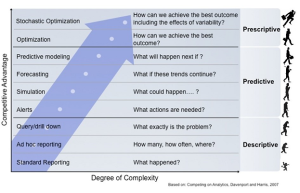
To generate a new schedule, there are 1,230 games to schedule each year. Each team has 41 home and 41 away games, and somewhere between 45 and 85 days when their home arena is available. The trick is to schedule each team so as to avoid long road trips, a densely-packed games, have more weekend games, make the games competitive, and several other criteria for a “good” schedule. The two aspects that are most important here are limiting fatigue, and competitive games. The league lowered the level of fatigue by lowering the number of back-to-back games and four games in five nights among other things. To make games competitive, the NBA tried to make sure that if a team was playing tired, i.e. on the second game of a back-to-back, so was their opponent.
What does this have to do with the Warriors? The Warriors were the beneficiaries of better scheduling (not unfair—just better). It allowed the best to rise to the top. The Warriors had 19 back-to-back games, and no four games in five nights sequence. By this measure, the 1995-1996 Bulls had a slightly harder schedule with 21 back-to-back games and one four games in five nights stretch. It is not much of a difference, but neither is the difference between 72 wins and 73 wins. Matt Winick’s scheduling prowess was close, but it was still improved on by prescriptive analytics (mathematical optimization). It is impressive that Mr. Winick came close to the optimal solution without analytics, but those small differences add up over a season and over a career.
The upshot is that the good teams this year had no excuse for losing to the bad teams. It is why the Spurs have also been doing so well and why the Lakers have had their worst season ever. So if you want to debate whether or not the 1995-1996 Bulls are better than the 2015-2016 Warriors, the scheduling is something you can point to and say, “but if the Bulls had had better scheduling…”
Balance Sheet Optimization: Clear, Crush, Offset, Exit, or Hold.
Balance Sheet Optimization: Clear, Crush, Offset, Exit, or Hold.
Is your company making the best decision possible?
Balance Sheet Optimization helps financial institutions determine what to do with their assets in order to better meet regulatory requirements and achieve higher profitability. Basel III, EMIR, and Dodd-Frank regulations have imposed higher capital ratios and reduced the risks that banks are allowed to take. But reducing the number of assets and the risk that banks take reduces the return on equity, putting pressure on profits and the ability to deliver returns to shareholders. In order to meet these capital requirements, banks must determine which trades to clear, crush, offset, or exit. They must also decide where to hold the assets that serve as hedges for a trade. Balance Sheet Optimization determines what to do with existing trades and where to hold the hedges in order to meet regulatory requirements and maintain profitability.
To register for this webinar go to:
Optimized Financial Systems Announces a Vendor Agreement with Ingram Micro
June 9, 2014- Today, Optimized Financial Systems announced a vendor agreement with Ingram Micro. Ingram Micro has global operations in more markets than any other technology and supply chain services company. Their global reach enables us to better serve our customers by leveraging their extensive sales and distribution network. Our strengths position us to meet the growth needs of our business partners around the world, combining geographic breadth with an understanding of local market nuances.
Ingram Micro offers Optimized Financial Systems a broad selection of programs and services, from financing, education, training and business development resources to marketing services and pre- and post-sale technical assistance.
Product Diversification – Ingram Micro offers a comprehensive portfolio of IT and mobility products, services and capabilities globally. Ingram Micro adds value to our comprehensive product portfolio via their suite of services, making them the one-stop shop for our company. Their unparalleled product selection and availability includes recent investments in specialty offerings and solutions in cloud, mobility, enterprise computing, data center, networking, automatic identification and data capture (AIDC), point-of-sale (POS), and consumer electronics.
Agility and Operational Efficiencies – With a wide geographic reach, Ingram Micro’s value is in enabling our business partners to become more efficient, knowledgeable and profitable. As a global company with a broad product portfolio, Ingram Micro offers economies of scale for small business, medium-sized and enterprise partners.
Lifecycle Services – Ingram Micro continues to lead the IT and mobility distribution markets as they evolve. As a leading third-party logistics (3PL) provider, they deliver the world’s most scalable multi-channel fulfillment solutions to product leaders in a variety of industries. The company offers a full range of value-added logistics services for technology and mobile markets, allowing our customers to focus on their products while we deliver them to the world.
Optimized Financial Systems. Solutions for Tomorrow. Engineered Today.
If you would like more information about this topic, please contact Andrea Onopa at 800-654-7959 or email at aonopa@optimizedfinancialsystems.com.
Optimized Financial Systems Announces Partnership with IBM
May 20, 2014- Today, Optimized Financial Systems announced a partnership with IBM. Optimized Financial Systems will be selling ILOG products including IBM ILOG CPLEX Optimization Studio, IBM ILOG Inventory and Product Flow Analyst, IBM ILOG LogicNet Plus XE, IBM Decision Optimization Center, and IBM ILOG Transportation Analyst. IBM ILOG Optimization products and solutions have broad applicability to a multitude of challenges in nearly every industry. They help organizations quickly determine how to most effectively allocate limited resources and to automatically balance trade-offs and business constraints, helping you achieve maximum operational efficiency and improved profitability. IBM ILOG Optimization products deliver measurable return on investment (ROI) through effective analytical decision-support solutions. IBM ILOG Optimization products and solutions support decision-making processes in situations where complexity and urgency limit the ability of human beings to consider multiple trade-offs. Users can implement better decisions faster by focusing their attention on critical complexities rather than on routine matters.
IBM ILOG Optimization products and solutions support decision- making processes in situations where complexity and urgency limit the ability of human beings to consider multiple trade-offs; product users can implement better decisions faster by focusing their attention on critical complexities rather than on routine matters.
IBM ILOG Inventory and Product Flow Analyst
Globalization and complexity in the supply chain make it difficult to identify the true drivers of inventory. IBM ILOG Inventory and Product Flow Analyst helps find the hidden drivers so that companies can prioritize improvement opportunities based on overall inventory impact. Global inventory optimization strategically positions raw materials, work in progress (WIP), and finished goods inventory throughout the supply chain to improve inventory turns, free up working capital, and increase cash flows.
IBM ILOG Inventory and Product Flow Analyst is a web-based, enterprise-inventory-optimization solution that helps manufacturers, retailers, and distributors manage their inventory from end-to-end. It handles both inbound/outbound and distribution-focused business models, helping companies answer a broad range of business questions, from determining the right inventory policies and strategic positioning of inventory to the ongoing setting of safety stocks and inventory levels in operational environments. Integral to an enterprise resource planning (ERP) system, it allows inventory planners to determine how much inventory should be kept in stock for each product on an ongoing basis.
IBM ILOG CPLEX Optimization Studio V12.6.1
IBM ILOG CPLEX Enterprise Server for Non-Production provides an ordering option for your development and testing environment with IBM ILOG CPLEX Optimization Studio V12.6.1. With the Processor Value Unit metric, you get a lower price point than the regular IBM ILOG CPLEX Enterprise Server to meet your nonproduction needs.
IBM ILOG CPLEX Optimization Studio offers an integrated modeling toolkit that enables rapid modeling and deployment of analytical optimization problems. It supports end-to-end mathematical modeling from prototyping through operational deployment. It includes CPLEX Optimizer solvers for mathematical programming and constraint programming that are robust and high speed providing confidence in accuracy and reliability. An open architecture facilitates interoperability with other modeling languages, tools, and systems.
IBM ILOG CPLEX Optimization Studio V12.6.1 now offers a trade-up option from Deployment Entry Edition Processor Value Unit (PVU) License to Deployment Edition Processor Value Unit (PVU) License.
Version 12.6.1 delivers:
- Improved solution times on difficult mixed-integer problems
- Improved solution times on scheduling problems
- An algorithm to provide a global optimum for problems with non- convex quadratic objectives
- An algorithm which harnesses compute clusters to solve mixed- integer problems
- Constraints to better model ordering relationships between operations and to easily specify highly combinatorial relationships
- Reorganization of parameters into a functional hierarchy
- Additional capability in the Integrated Development Environment
- Updated price metrics and structures
- Floating User Single Session (FUSS) licensing
IBM Decision Optimization Center
In response to a shift in the market toward line-of-business adoption of enterprise decision-making solutions and applications, the product name, IBM ILOG ODM Enterprise, is renamed IBM Decision Optimization Center. Decision Optimization Center is a flexible, optimization-powered platform that delivers optimization across many business functions through a common architecture that provides the intelligence needed to help transform data insights into action. Unlike other decision-support packages, custom solutions, and development environments, Decision Optimization Center gives:
- Enterprises the flexibility and speed to make and validate forward-looking decisions through a common portal for adopting or building optimization models for enterprise deployment.
- Lines of business the power to transform analytic insights into prescribed planning and scheduling, supply chain, and asset utilization actions that generate competitive advantage.
- IT a modernized, flexible deployment architecture for implementing enterprise analytic applications and business value solutions across the global value chain.
- Solution developers a CPLEX-powered development platform for creating innovative decision support applications by effectively applying operations research methods.
Key features in V3.8 include:
- Performance and scalability: Lower latency in the business user interface helps improve the user experience when working with large data sets.
- Rapid and flexible application development: The use of scripting helps reduce the time and effort required to customize data models and views.
- An effective business interface: The ability to define user roles and rights helps planners differentiate roles in the planning process to support organizational business processes. Enhancements in this release allow planners to see or interact only with data relevant to their role such as world-wide versus local planning.
- Ease of use: Enhancements to the Gantt chart component enable business users to move activities within a schedule interactively in real time.
- Flexible architecture: A basic representational state transfer (REST) API helps facilitate application web deployment, especially for integration requirements such as data access and job control.
IBM ILOG ODM Enterprise V3.8
IBM Optimization helps businesses determine how to most effectively allocate limited resources and to automatically balance trade-offs and business constraints to achieve maximum operational efficiency. IBM Optimization delivers measurable return on investment (ROI) through effective, analytical decision-support solutions. IBM Optimization supports decision-making processes in situations where complexity and urgency mandate solutions that can quickly and automatically analyze the operational impact of numerous business decisions.
IBM ILOG Optimization Decision Manager (ODM) Enterprise V3.7 offers a platform for advanced analytics solutions based on optimization, with out-of-the-box features such as ‘what-if’ analysis, user-friendly GUIs, and a repeatable implementation process for deploying enterprise-wide, decision support.
IBM ILOG Optimization Decision Manager Enterprise V3.7 helps address the needs of:
- Line-of-business decision makers seeking to improve business operations and planning to achieve better resource utilization within their specific industry domains
- Information technology specialists seeking to provide dynamic, collaborative, connected decision support that influences information resources across the enterprise
- Analytics experts seeking to rapidly develop and deploy optimization decision support applications
- Companies and organizations “competing on analytics” by making customer-centric, fact-based, data-driven decisions who need extensible, decision management solutions
- Organizations focused on improving operational and commercial efficiency
Platform-based, optimization solutions often make it easier for line-of-business decision makers to create, share, and deploy custom plans and schedules across the extended enterprise. These solutions help them to make the best use of limited resources while managing risk and maximizing value.
Industry accelerators such as Empty Container Repositioning or Complex Project Scheduling, based on ODM Enterprise, can be tailored to fit business processes and practices. This enables “what-if” analysis, and support for automatic or guided resolution of trade offs and conflicting business objectives.
ODM Enterprise enhancements include:
- Synchronized support for the Domain Object Model to link enterprise application data with effective decision support
- Built-in support for date-related data types in the Application Data Model, views, and optimization models
- An API to store and restore ODM Studio view configurations
- Support for Linux SUSE and RHEL (applies to IBM ILOG ODM Enterprise Data Server and IBM ILOG ODM Enterprise Optimization Server only)
- Built-in support for Gantt view that is configurable from the ODM Enterprise IDE as existing simple table views or pivot table views
- An industry accelerator for the mining industry, Mine to Ship Optimization. For more information, refer to
http://www-01.ibm.com/software/data/information-agenda/ catalog/profiles/Opt_Mind_to_Ship_IND_12.html
These enhancements help businesses improve decision making through the application of advanced analytics on top of existing IT solutions. Ready-made industry connectors based on pre-built, validated assets for Industrial Manufacturing and Travel & Transportation industries are also available. These assets provide an advanced starting point to develop industry-specific, custom planning and scheduling solutions that are tailored to fit your business.
IBM ODM Enterprise V3.7 helps line-of-business decision makers who need to:
- Improve business operations and planning through better resource utilization within their specific industry domains.
- Provide dynamic, collaborative, connected decision support by influencing information resources across the enterprise.
- Develop and deploy planning and scheduling applications tailored to fit the organization.
- Make fact-based, data-driven decisions quickly and reliably in time critical situations.
- Improve operational and commercial efficiency.
IBM Optimization Solutions Accelerator, an enhanced feature, helps enable:
- Cost-effective and lower risk development and deployment of industry-specific solutions
- Enhanced globalization
Notes:
- Optimization Programming Language
- Optimization Decision Manager
Optimized Financial Systems. Solutions for Tomorrow. Engineered Today.
If you would like more information about this topic, please contact Andrea Onopa at 800-654-7959 or email at aonopa@optimizedfinancialsystems.com.
###
Fantasy Football Prediction Using Vectorial ARMA Models
| Fantasy Football Prediction Using Vectorial ARMA Models |
Abstract
Fantasy Football is the most popular fantasy sport in the United States with estimates of 33 million participants every year. In addition to league fees that are paid to internet providers, many leagues have their own pool of money with the winner taking the lion’s share. The Fantasy Sports Trade Association (FSTA) estimated in 2013 that $1.18 billion changes hands within leagues every year (Green, 2014). In addition to the financial stakes is personal pride; no one wants to lose.
In order to gain an edge on their fellow fantasy league managers, team managers can turn to many web sites for guidance. A simple search on bing.com returns 63,000 results for the term “Fantasy Football 2014 Rankings.” There is no shortage of sites offering advice on how to draft, who to draft, and when to draft. At the core of this process is estimating how much a given player will score in each game and over the course of a season.
This paper discusses techniques for using Vectorial ARMA models to improve the predictions of quarterback fantasy statistics.
Introduction
Fantasy football began in 1962 when Wilfred Winkenbach with some colleagues developed a system and rules that led to the formation of modern fantasy football (Hunt, 2014). The growth of the game was slow due to the manual nature of entering and keeping track of scores. The growth of fantasy football took off in the late 1990’s when the popularity of the internet and the automation of administrative duties made it possible for millions of fans to just choose their teams without having the administrative burden. Today, 33 million people play every year.
In fantasy football regular people get to pretend to be team owners. They choose their players and assemble a team of stars. A group of friends can form a league and compete against each other. Typically they pay a website an annual fee to host the league and draft process and compete against each other in a round-robin format for the first 12 or 13 weeks of the season. At the end of the 12 weeks, the top four teams go into the playoffs. The best teams compete against each other in multi-week rounds, and in the 16th week, the league champion is crowned. There are 17 weeks in the NFL season, but most leagues stop after 16 because many stars do not play the 17th week if their teams have already secured a spot in the real playoffs.
Fantasy teams score points by accumulating various statistics from the real-life performances of players on the field. Each team usually includes a quarterback, three wide receivers, two running backs, a tight end, a kicker, and a defense (an entire team is chosen). An entire team is made up of 16 different players, and the manager selects which players will “play” each week. If the active players score certain statistics, their managers are rewarded with points. The team with the most points wins the matchup and each manager accumulates a win-loss record, which makes him/her eligible for the playoffs and a portion of the league payout.
The team manager chooses the players on their team through a draft process. The two common draft procedures are the snake draft and the auction draft. In the snake draft, the managers take turns making picks. Prior to the draft an order is set. To make the draft process fair, the manager that picked first in the first round, picks last in the second round, and then picks first again in the third round, etc. The image below shows a typical snake draft.
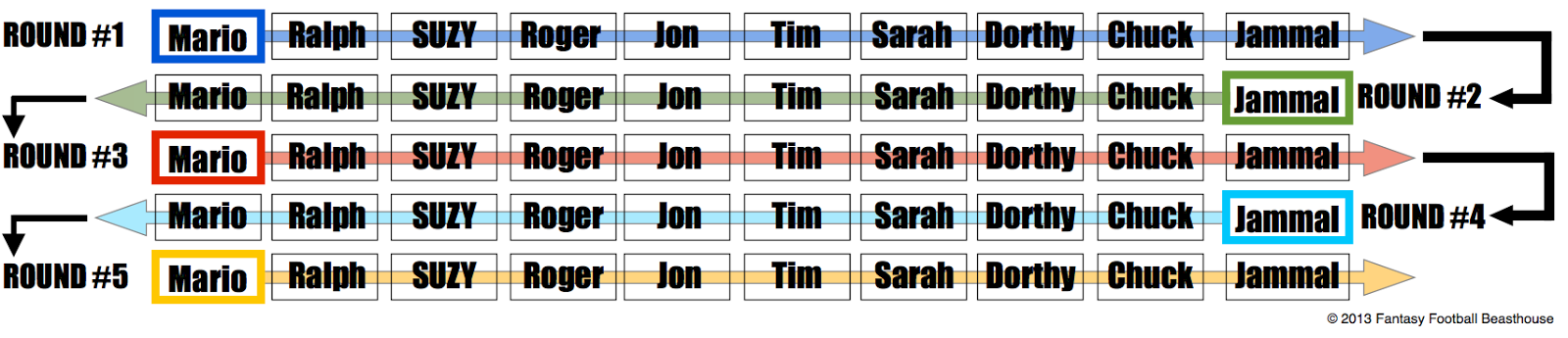
In a snake draft it is important to choose the player that will improve the team’s performance the most that is not likely to be available the next time the team manager is able to draft. Determining which players will not be available gets more difficult in later rounds, but it does not matter as much either. The marquee players always go in the first two or three rounds. Even if an estimate of a player’s worth is off a few positions the player is still not likely to be available the next time the manager drafts. In many leagues, certain positions will not be taken before certain rounds. So even if a player is more valuable, it helps to know that he may be available the next round, and can be safely undrafted until the next opportunity arises.
The alternative type of draft is the auction draft. In an auction draft, each player receives a budget, similar to the NFL’s salary cap. The manager’s take turns choosing a player and the managers bid on the player. The highest bid for a player wins. There is a strategy involved in this method as well. It may be that one manager wants to force another manger to overbid on a certain player. This will consume more of the opposing manager’s budget and lower the price for following players.
Fantasy football, like other fantasy sports, allows the fans to more actively participate in the sport. Whereas in the days before fantasy football most fans knew about their own team, and could name a few stars from the rest of the National Football League (NFL), fantasy football requires a deeper knowledge of the players in the league. In a league with 12 teams and 16 players per team, team managers need to know at least 192 of the players in the league. It also means that on any given night, a team manager will have a rooting interest in several other games. This is good business for the NFL.
For the team managers, being good at fantasy football means the owner knows more about football than the other owners in the league. Part of each year’s draft preparation is to determine which players are likely to score the most fantasy points. Most fantasy football web sites provide their own predictions for each player. The methodology behind these projections is opaque. The objective in this paper is to apply time series analysis to football statistics in order to come up with better predictions and a better overall team.
Method
The first part of this analysis was to get the data to use within MATLAB. For this, I went to a web site called FFToday.com. They have weekly statistics and fantasy scoring for every player at every position going back to the year 2,000. The data is in table format. This can be copied and pasted into Microsoft Excel, but requires manipulation within Excel in order make it ready to store in a database. Additionally, copying and pasting the results for 14 seasons for 6 different positions would take several days and is subject to manual error. Instead, I created a Python model that uses the built-in urllib to “screen scrape” the data and load it into a sqlite database. This procedure could load the 14 seasons into the database in about 30 minutes. In all, over 100,000 rows of data were downloaded.
Given the complexity of analyzing the factors contributing to the scoring of every position, I changed the focus to just quarterbacks. For the quarterbacks, I had 16,123 rows of data compiled by 247 different quarterbacks. This is an average of only 65 games per player. This is not enough data to complete a time series analysis. Additionally, many of those players only played a few games in a season and mostly scored 0 points each game. Only four quarterbacks had close to 200 games of history, these were Peyton Manning (195), Matt Hasselbeck (210), Tom Brady (210), and Drew Brees (195). Given the need for close to 200 samples, and an average career that is only 1/3 of that, I searched for another method.
Rather than model each quarterback, I flipped the problem on its side. Instead of modeling what a quarterback scored over time, I modeled what quarterbacks scored over time against a specific team.
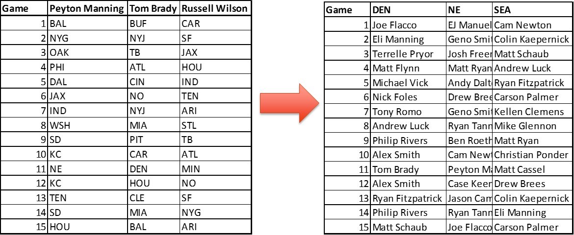
To account for the differences in the quarterbacks playing against each team, the quarterback’s average from the prior season was subtracted from the score. I subtracted the average of the residuals to get a time series for each team with a mean of 0.
The residuals all appear to be random data, and the correlated residuals did not show any abnormal patterns.
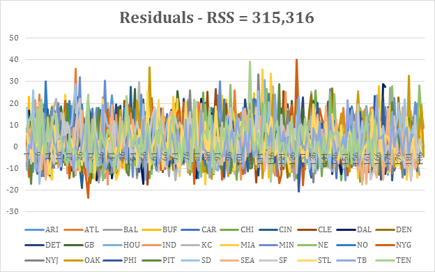
Residuals for each team
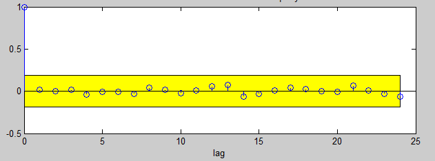
Correlated residuals for a sample team.
In order to get a base model, I ran the Postulate ARMA Matlab script. Most models were ARMA (1,1) and typically looked like white noise. There were some exceptions, such as Detroit, Denver, and Cleveland, which had higher order models. The results are in Appendix B. Given the normalizing process worked so well, so that most of the data could be seen as white noise, I modified the Postulate script to try and see if a higher MA order was possible. After the AR order is determined, Postulate checks to see if it can reduce the MA order further. Instead of starting from (m,n) and working back to (m,0), I made the incumbent model (m,20) and worked backwards. In most cases the final model was still ARMA (1, 1). One exception is Philadelphia with ARMA (3, 10). All other examples had MA orders lower than their AR orders.
Once the base model was determined, I experimented with using other time series to determine improve the forecast. The potential new time series were the following:
- Sacks: This is when the defensive team tackles the quarterback before he can pass it. The reasoning behind its importance is that a quarterback can get hurt, and will be more cautious or throw the ball away rather than be sacked again.
- Interceptions: This is when the defensive team catches a pass from the quarterback. An interception affects the quarterback’s confidence and takes the quarterback off the field so he cannot score more points.
- Fumbles Recovered: This happens when a player drops the ball and the play has not stopped, but the defense recovers the ball.
- Rushing Attempts: This is the number of attempts by the quarterback’s team to rush the ball. This happens when the quarterback chooses to hand the ball off instead of throwing it. The quarterback does not accumulate any statistics when this happens. It is less risky, but may not yield as many gains down the field.
- Rushing Touchdowns: This happens on a rushing play and the running back scores a touchdown. Again, the quarterback does not gain any point on this play.
Though it is likely that all five of these time series could contribute to improving the forecast of a quarterback’s scoring, I chose to only include two of the new time series in the analysis. These were the sacks and interceptions. These two time series are consistent from one observation to the next because it is the same defensive team responsible for the statistics. For this analysis I used the ARMA given by the modified postulate script and changed the order for the sacks and interceptions time series inputs.
When trying to add an order one ARV term to the model for either sacks or interceptions, the results showed no improvement in the reduction of the residual sum of squares (RSS). When combining the two, it did show some improvement, but not enough to be statistically significant. As a result, I experimented with ARV (2, 2) and ARV (3, 3). Both of these yielded a few significant improvements for some teams, but most teams still worked best with just their standard ARMA models and not ARMAV. The results of the F Tests for the ARMAV examples are in Appendix A.
Results
In 2012, with the exception of the top quarterback, the difference in the average number of fantasy points scored per game by each quarterback was less than one point per game. The average number of points scored by the number two quarterback in 2012, Tom Brady was 25.52. The 12th quarterback, Russell Wilson, was 20.32. In the NFL, the schedules adjust from year to year, so that a team that did poorly the year before will face other teams that did poorly the year before. The upcoming schedule for a quarterback can be important. It may only affect the points by less than a point per game, but this difference can move the quarterback up or down two to three spots. Armed with this knowledge, a fantasy football manager can pay less or draft later if he knows a player will exceed the expectations that most others have put upon him.
The following table includes the forecasts for the top 12 quarterbacks of 2013.
| Player | Team | Actual Average | Forecast | Actual Rank | Forecast Rank |
| Peyton Manning | DEN |
31.18667 |
26.49 |
1 |
5 |
| Drew Brees | NO |
26.4 |
28.88 |
2 |
1 |
| Matthew Stafford | DET |
23.54667 |
24.67 |
3 |
8 |
| Andy Dalton | CIN |
23.13333 |
23.19 |
4 |
10 |
| Cam Newton | CAR |
22.5 |
28.09 |
5 |
2 |
| Philip Rivers | SD |
22.39333 |
20.21 |
6 |
12 |
| Ben Rothlisberger | PIT |
21.84 |
24 |
7 |
9 |
| Andrew Luck | IND |
21.78 |
25.59 |
8 |
6 |
| Matt Ryan | ATL |
21.37 |
26.94 |
9 |
4 |
| Tony Romo | DAL |
21.34 |
25.49 |
10 |
7 |
| Russell Wilson | SEA |
21.30667 |
22.7 |
11 |
11 |
| Tom Brady | NE |
20.62667 |
27.43 |
12 |
3 |
The table also shows the actual averages, the rank of the player in reality as well as the rank in the forecast. An ideal forecast would match up the forecasts with the actual results. A second option is for the forecast rankings to match up with the actual rankings. This can provide a relative scale for comparison if not an absolute one.
Further Study
The base ARMAV models developed here only begin to analyze the possibilities for improving forecasting of fantasy sports statistics. The likelihood is that a much larger ARMAV model that incorporates the influence of quarterback statistics on other player’s statistics as well as other player’s statistics on the quarterback. A second challenge is finding a framework for evaluating the large number of combinations of orders for the different inputs and outputs of an ARMAV model.
Given the large interest in fantasy football and other fantasy sports in the United States, increasing the scope of the analysis could yield promising results.
Appendix A: F Statistics for ARMAV (M,N,2,2) and (M,N,3,3) Models
The following tables show the results of the F Tests for the ARMAV models. Due to numerical instability some results were actually worse in the unrestricted models. The first table shows the results of adding two orders for both the sacks and interceptions to help predict the quarterback statistics. The second set of statistics shows the results when the order is increased to three for each the sacks and interceptions.
| Team | Restricted Parameters | Unrestricted Parameters | Observations | Restricted Sum RSS | Unrestricted Sum RSS | F Statistic | Significance |
| ARI |
3 |
6 |
172 |
10285.4851 |
10195.3819 |
0.4890 |
0.2975 |
| ATL |
3 |
6 |
174 |
11360.0211 |
11268.3021 |
0.4558 |
0.2771 |
| BAL |
3 |
6 |
171 |
10696.9480 |
10481.1823 |
1.1322 |
0.5916 |
| BUF |
3 |
6 |
168 |
12953.0207 |
12304.4148 |
2.8465 |
0.8725 |
| CAR |
3 |
6 |
171 |
8936.3690 |
8581.0042 |
2.2777 |
0.8203 |
| CHI |
3 |
6 |
170 |
12287.2196 |
11526.2334 |
3.6092 |
0.9152 |
| CIN |
3 |
6 |
168 |
9464.9076 |
8431.5749 |
6.6180 |
0.9752 |
| CLE |
6 |
8 |
169 |
10764.9152 |
10246.3073 |
1.3581 |
0.6649 |
| DAL |
3 |
6 |
156 |
10063.3818 |
9723.9933 |
1.7451 |
0.7430 |
| DEN |
7 |
11 |
171 |
10004.0909 |
8892.8525 |
2.8562 |
0.9416 |
| DET |
6 |
8 |
172 |
10237.8159 |
10489.1036 |
-0.6548 |
N/A |
| GB |
3 |
7 |
170 |
10784.1283 |
10119.0447 |
3.5711 |
0.9249 |
| HOU |
3 |
6 |
142 |
7220.3740 |
6668.7833 |
3.7496 |
0.9209 |
| IND |
3 |
6 |
156 |
10010.1706 |
9256.0704 |
4.0735 |
0.9323 |
| KC |
3 |
6 |
171 |
12415.4241 |
12273.4306 |
0.6363 |
0.3815 |
| MIA |
3 |
7 |
173 |
16339.5905 |
15919.5163 |
1.4601 |
0.6947 |
| MIN |
3 |
6 |
171 |
12305.8284 |
11959.3659 |
1.5933 |
0.7133 |
| NE |
4 |
8 |
173 |
11245.5795 |
11470.3170 |
-0.8082 |
N/A |
| NO |
3 |
6 |
170 |
9977.7447 |
9838.1556 |
0.7756 |
0.4512 |
| NYG |
3 |
6 |
155 |
12463.7069 |
12157.5940 |
1.2505 |
0.6282 |
| NYJ |
3 |
6 |
171 |
11395.4468 |
11490.7386 |
-0.4561 |
N/A |
| OAK |
3 |
6 |
175 |
11947.5855 |
11571.3831 |
1.8315 |
0.7581 |
| PHI |
8 |
14 |
157 |
7677.0347 |
7089.3913 |
1.4817 |
0.7516 |
| PIT |
3 |
6 |
166 |
9463.9612 |
9310.3132 |
0.8802 |
0.4976 |
| SD |
3 |
6 |
174 |
12082.6343 |
11632.3226 |
2.1679 |
0.8071 |
| SEA |
6 |
9 |
171 |
10448.4292 |
10379.1815 |
0.1801 |
0.0247 |
| SF |
3 |
8 |
174 |
10785.3918 |
10391.5605 |
2.0971 |
0.8210 |
| STL |
3 |
6 |
170 |
9744.4409 |
8788.2954 |
5.9476 |
0.9686 |
| TB |
4 |
8 |
168 |
10851.8750 |
10833.9241 |
0.0663 |
0.0096 |
| TEN |
8 |
9 |
153 |
8372.5216 |
8716.8504 |
-0.7110 |
N/A |
Order 2 for sacks and interceptions
| Team | Restricted Parameters | Unrestricted Parameters | Observations | Restricted Sum RSS | Unrestricted Sum RSS | F Statistic | Significance |
| ARI |
3 |
8 |
172 |
10285.48506 |
9925.733651 |
1.9814 |
0.8046 |
| ATL |
3 |
8 |
174 |
11360.02105 |
11051.77038 |
1.5433 |
0.7232 |
| BAL |
3 |
8 |
171 |
10696.94803 |
9985.920666 |
3.8687 |
0.9441 |
| BUF |
3 |
8 |
168 |
12953.0207 |
12029.3453 |
4.0952 |
0.9508 |
| CAR |
3 |
8 |
171 |
8936.369026 |
8465.145136 |
3.0245 |
0.9064 |
| CHI |
3 |
8 |
170 |
12287.21957 |
11852.56084 |
1.9803 |
0.8044 |
| CIN |
3 |
8 |
168 |
9464.907607 |
8590.749882 |
5.4270 |
0.9751 |
| CLE |
6 |
10 |
169 |
10764.91525 |
11093.83048 |
-0.7857 |
N/A |
| DAL |
3 |
8 |
156 |
10063.38175 |
9655.470255 |
2.0842 |
0.8193 |
| DEN |
7 |
13 |
171 |
10004.09094 |
8832.746985 |
2.9933 |
0.9581 |
| DET |
6 |
10 |
172 |
10237.81591 |
9773.673713 |
1.2822 |
0.6534 |
| GB |
3 |
9 |
170 |
10784.12825 |
10474.49471 |
1.5864 |
0.7402 |
| HOU |
3 |
8 |
142 |
7220.37405 |
6544.540991 |
4.6126 |
0.9628 |
| IND |
3 |
8 |
156 |
10010.17062 |
9533.604287 |
2.4661 |
0.8633 |
| KC |
3 |
8 |
171 |
12415.42412 |
11885.21505 |
2.4239 |
0.8591 |
| MIA |
3 |
9 |
173 |
16339.59053 |
15688.51971 |
2.2687 |
0.8505 |
| MIN |
3 |
8 |
171 |
12305.82836 |
11763.92797 |
2.5028 |
0.8668 |
| NE |
4 |
10 |
173 |
11245.57951 |
11411.25086 |
-0.5916 |
N/A |
| NO |
3 |
8 |
170 |
9977.744654 |
9628.754156 |
1.9572 |
0.8009 |
| NYG |
3 |
8 |
155 |
12463.70693 |
12097.02572 |
1.4853 |
0.7096 |
| NYJ |
3 |
8 |
171 |
11395.44683 |
11167.01181 |
1.1115 |
0.6003 |
| OAK |
3 |
8 |
175 |
11947.5855 |
11202.88246 |
3.7004 |
0.9383 |
| PHI |
10 |
14 |
157 |
7677.034712 |
7446.771538 |
0.4422 |
0.0993 |
| PIT |
3 |
8 |
166 |
9463.961223 |
8788.332012 |
4.0489 |
0.9495 |
| SD |
3 |
8 |
174 |
12082.63432 |
11537.14403 |
2.6162 |
0.8769 |
| SEA |
6 |
11 |
171 |
10448.42919 |
10325.41878 |
0.3177 |
0.0856 |
| SF |
3 |
10 |
174 |
10785.39175 |
10359.04634 |
2.2499 |
0.8549 |
| STL |
3 |
8 |
170 |
9744.440851 |
8732.685735 |
6.2564 |
0.9829 |
| TB |
4 |
10 |
168 |
10851.875 |
10571.65603 |
1.0470 |
0.5694 |
| TEN |
8 |
11 |
153 |
8372.521556 |
8191.07695 |
0.3932 |
0.0977 |
Order 3-3 for sacks and interceptions
Appendix B: Order for Quarterback ARMA Model
| M | N | |
| ARI |
1 |
1 |
| ATL |
1 |
1 |
| BAL |
1 |
1 |
| BUF |
1 |
1 |
| CAR |
1 |
1 |
| CHI |
1 |
1 |
| CIN |
1 |
1 |
| CLE |
3 |
2 |
| DAL |
1 |
1 |
| DEN |
4 |
2 |
| DET |
3 |
2 |
| GB |
1 |
1 |
| HOU |
1 |
1 |
| IND |
1 |
1 |
| KC |
1 |
1 |
| MIA |
1 |
1 |
| MIN |
1 |
1 |
| NE |
2 |
1 |
| NO |
1 |
1 |
| NYG |
1 |
1 |
| NYJ |
1 |
1 |
| OAK |
1 |
1 |
| PHI |
3 |
10 |
| PIT |
1 |
1 |
| SD |
1 |
1 |
| SEA |
4 |
1 |
| SF |
1 |
1 |
| STL |
1 |
1 |
| TB |
2 |
1 |
| TEN |
4 |
3 |
References
Green, M. (2014, 05 08). NFL’s Shadow Economy of Gambling and Fantasy Footlball is a Multibillion Dollar Business. Retrieved from The Daily Beast: http://www.thedailybeast.com/articles/2012/10/06/nfl-s-shadow-economy-of-gambling-and-fantasy-football-is-a-multibillion-dollar-business.html
Hunt, M. (2014, 05 08). How Fantasy Football Works. Retrieved from How Stuff Works: http://entertainment.howstuffworks.com/fantasy-football1.htm
KAz, J. (2014, 05 08). Fantasy Football 101 – What is a Fantasy Football Snake Draft? . Retrieved from Fantasy Football Beast House: http://www.fantasyfootballbeasthouse.com/2013/06/what-is-a-fantasy-football-snake-serpentine-draft.html